Poisson Process simplified

Statistics cab also be a good ally if we just try to focus on concepts and don’t much bothered about the derivations—though it requires a lot of patience to understand the derivations but it is not mandatory to know all of it to take advantage of the concepts, we should understand derivations on need to know basis and focus more on concepts. Here, we will try to unfold Poisson process for beginners in below mentioned steps—

1. Poisson process definition.
2. Real word examples of Poisson process.
3. How can we identify a process as a Poisson process.
4. Correlation between Poisson and Exponential process. 
5. Metrics related to Poisson and Exponential process to understand the process more in detail. 
6. Python code to calculate calculate metrics related to Poisson and Exponential process. 

So let’s get started to deep dive and learn in depth concepts. 

“A Poisson process is a simple and widely used stochastic process for modelling the times at which arrivals enter a system.”

Let’s try to understand what we just said—A Poisson Process is a model for series of discrete event where exact timing of events is random but average time between events is known. For example, Number of cars passing by a police station each hour can be a Poisson process. Below are some of the characteristics of a Poisson process.

1. Events are independent of each other. The occurrence of one event does not affect the probability another event will occur—passing of one car doesn’t affect the probability of passing other car.
2. The average rate (events per time period) is constant—It is calculated on the basis of monitoring for a long period of time.
3. Two events cannot occur at the same time—though in our scenario two cars can be passed at the same time, but for experiment point of view we can consider it as two events will not occur at same time.

Suppose that we would like to model the arrival of events that happen completely at random at a rate λ per unit time. Here is one way to do this. At time t=0, we have no arrivals yet, so N(0)=0. We now divide the half-line [0,∞) to tiny sub intervals of length δ as shown in Figure.

Each sub interval corresponds to a time slot of length δ. Thus, the intervals are (0,δ], (δ,2δ], (2δ,3δ], . More generally, the kth interval is ((k−1)δ,kδ]. So considering the previous example, it may be possible in an interval no car crosses the police station, but it could also be possible to have back to back cars crosses the police station in an interval. 

Other examples of Poisson process are customers calling help centre, visitors to a website, manufacturing issues, patients arriving to hospital etc. Let’s model customers calling help centre as a Poisson distribution process as two customers callings are independent to each other, the average rate of customers calling per hour is constant and two customers can not call at the same time—assuming we have only one executive to pick up the call. 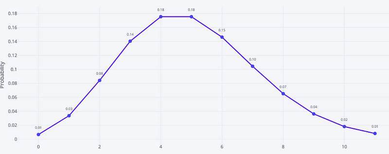Below is the probability distribution of customers calling each hour. 

So based on above figure we can say—Probability of getting 0 call in an hour is .01, Probability of getting 1 call in an hour is .03, Probability of getting 2 call in an hour is .08, Probability of getting 3 call in an hour is .14 etc. and sum of all the probabilities will be 1.

Now, the question is how can we identify above probabilities for a process— To do that, first we need to identify if a process is a Poisson process or not—based on previously discussed criteria, Once a process is identified as a Poisson process, we can calculate different metrics related to Poisson process and take advantage of the derivations. 

Here we can understand two things from the above figure, 

1. Number of events in a fixed time interval follows Poisson distribution. 
2. Time elapsed between two successive events in Poisson process follows exponential distribution.

Given events whose count per time follows a Poisson distribution, then the time between events follows an exponential distribution with the same rate parameter λ. This correspondence between the two distributions is essential to name-check when discussing either of them.

Let’s now try to calculate metrics associated with these distributions.

1. Probability of getting k events in an interval— The only parameter of the Poisson distribution is λ, the event rate (or rate parameter)— This represents the expected number of events in an interval.

λ = (events/interval) * interval length

Let’s take average rate as 10 customers calling each hour, Then, λ (or expected number of events in an interval) are—

λ = 10/60*60 =10 customers expected

Now let’s try to see what will be the probability that x customers will call in an hour, it is also called as Poisson distribution probability function—

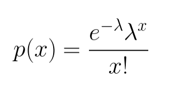
Now take some examples and try to see what does it mean, Let’s try to see what is the probability that 5 customers will call in an hour—P(5)= .037. So there is .037 probability that we will get exactly 5 call in an hour. 

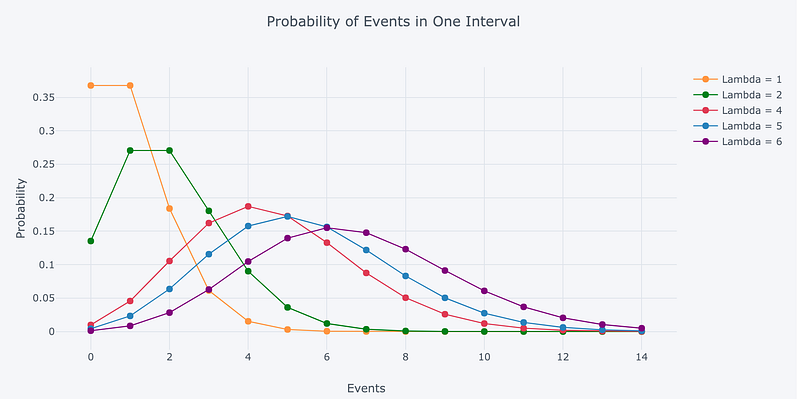
As we change the rate parameter, λ, we change the probability of seeing different numbers of events in one interval. The below graph is the probability mass function of the Poisson distribution showing the probability of a number of events occurring in an interval with different rate parameters.

Let’s try to see it by code—

import pandas as pd
import numpy as np

from scipy.special import factorial
np.random.seed(42)

import plotly.plotly as py
import plotly.graph_objs as go
from plotly.offline import iplot
import cufflinks as cf

events_per_minute = 1/6
minutes = 60

# Expected events
lam = events_per_minute * minutes

k = 5
p_k = np.exp(-lam) * np.power(lam, k) / factorial(k)
print(f'The probability of {k} customers call in {minutes} minutes is {100*p_k:.2f}%.')

2. Waiting time between events in a Poisson Process is decaying exponential —or follows exponential distribution 

An interesting part of a Poisson process involves figuring out how long we have to wait until the next event (this is sometimes called the inter arrival time). Consider the situation: Customers call every 10 minutes on average. If we arrive at a random time, how long can we expect to wait to see the next call? We won’t go into the derivation (it comes from the probability mass function equation, as promised), but the time we can expect to wait between events is a decaying exponential, or called exponential distribution. The probability of waiting a given amount of time between successive events decreases exponentially as the time increases. The following equation shows the probability of waiting more than a specified time.

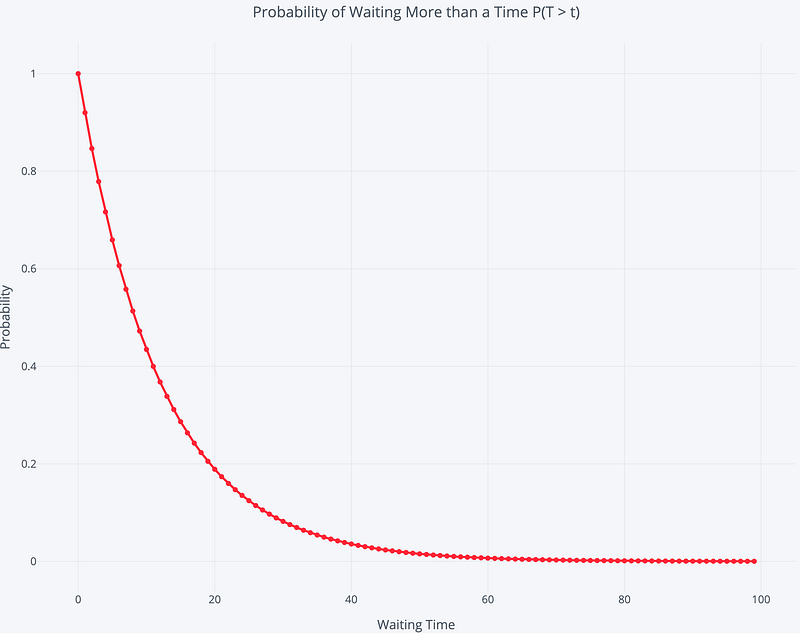
With our example, we have 1 event/10 minutes, and if we plug in the numbers we get a 60.65% chance of waiting > 5 minutes (We need to note this is between each successive pair of events. The waiting times between events are memory less, so the time between two events has no effect on the time between any other events).

Let’s try to see it with python code—

import pandas as pd
import numpy as np

from scipy.special import factorial
np.random.seed(42)

import plotly.plotly as py
import plotly.graph_objs as go
from plotly.offline import iplot
import cufflinks as cf
cf.go_offline()
cf.set_config_file(world_readable=True, theme='pearl')

events_per_minute = 1/10
t = 5
p_k = np.exp(-events_per_minute*t) 
print(f'The probability of {k} customers call in {minutes} minutes is {100*p_k:.2f}%.')

Hope, now you have understood what a Poisson process is and how Poisson process is correlated to Exponential process and once a process is identified as Poisson process what are the metrics you can calculate associated to that process. 

Please hit like if you enjoyed the blog, that would encourage us to come up with more interesting topics and explain them in-depth here.