


The huge amount of data that we’re generating every day, has led to an increase of the need for advanced Machine Learning Algorithms. One such well-performed algorithm is the K Nearest Neighbour algorithm.
In this blog on KNN Algorithm In R, we will understand what is KNN algorithm in Machine Learning and its unique features including the pros and cons, how the KNN algorithm works, an essay example of it, and finally moving to its implementation of KNN using the R Language.
It is quite essential to know Machine Learning basics. Here’s a brief introductory section on what is Machine Learning and its types.
Machine learning is a subset of Artificial Intelligence that provides machines the power to find out automatically and improve from their gained experience without being explicitly programmed.
There are mainly three types of Machine Learning discussed briefly below:
-
Supervised Learning: It is that part of Machine Learning in which the data provided for teaching or training the machine is well labeled and so it becomes easy to work with it.
-
Unsupervised Learning: It is the training of information using a machine that is unlabelled and allowing the algorithm to act on that information without guidance.
-
Reinforcement Learning: It is that part of Machine Learning where an agent is put in an environment and he learns to behave by performing certain actions and observing the various possible outcomes which it gets from those actions.
Now, moving to our main blog topic,
What is KNN Algorithm?
KNN which stands for K Nearest Neighbor is a Supervised Machine Learning algorithm that classifies a new data point into the target class, counting on the features of its neighboring data points.
Let’s attempt to understand the KNN algorithm with an essay example. Let’s say we want a machine to distinguish between the sentiment of tweets posted by various users. To do this we must input a dataset of users’ sentiment(comments). And now, we have to train our model to detect the sentiments based on certain features. For example, features such as labeled tweet sentiment i.e., as positive or negative tweets accordingly. If a tweet is positive, it is labeled as 1 and if negative, then labeled as 0.
Features of KNN algorithm:
-
KNN is a supervised learning algorithm, based on feature similarity.
-
Unlike most algorithms, KNN is a non-parametric model which means it does not make any assumptions about the data set. This makes the algorithm simpler and effective since it can handle realistic data.
-
KNN is considered to be a lazy algorithm, i.e., it suggests that it memorizes the training data set rather than learning a discriminative function from the training data.
-
KNN is often used for solving both classification and regression problems.
If you want to learn the Concepts of Data Science Click here
Disadvantages of KNN algorithm:
-
After multiple implementations, it has been observed that KNN algorithm does not work with good accuracy on taking large datasets because the cost of calculating the distance between the new point and each existing points is huge, and in turn it degrades the performance of the algorithm.
-
It has also been noticed that working on high dimensional data is quite difficult with this algorithm because the calculation of the distance in each dimension is not correct.
-
It is quite needful to perform feature scaling i.e., standardization and normalization before actually implementing KNN algorithm to any dataset. Eliminating these steps may lead to wrong predictions by KNN algorithm.
-
Sensitive to noisy data, missing values and outliers: KNN is sensitive to noise in the dataset. We need to manually impute missing values and remove outliers.
KNN Algorithm Example
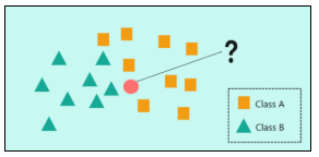
In order to make understand how KNN algorithm works, let’s consider the following scenario:
In the image, we have two classes of data, namely class A and Class B representing squares and triangles respectively.
The problem statement is to assign the new input data point to one of the two classes by using the KNN algorithm
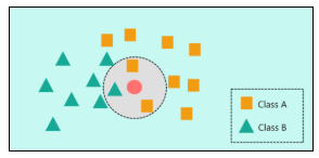
The first step in the KNN algorithm is to define the value of ‘K’ which stands for the number of Nearest Neighbors.
In this image, let’s consider ‘K’ = 3 which means that the algorithm will consider the three neighbors that are the closest to the new data point. The closeness between the data points is calculated either by using measures such as Euclidean or Manhattan distance. Now, at ‘K’ = 3, two squares and 1 triangle are seen to be the nearest neighbors. So, to classify the new data point based on ‘K’ = 3, it would be assigned to Class A (squares).
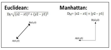
Ways to measure the new data point and nearest data points:
Euclidian Distance: It always gives the shortest distance between the two points.
Manhattan Distance: To measure the similarity, we simply calculate the difference for each feature and add them up.
Practical Implementation of KNN Algorithm in R
Problem Statement: To study a bank credit dataset and build a Machine Learning model that predicts whether an applicant’s loan can be approved or not based on his socio-economic profile.
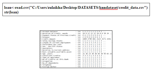
Step 1: Import the dataset and then look at the structure of the dataset:
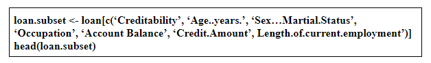
Step 2: Data Cleaning
From the structure of the dataset, we can see that there are 21 predictor variables but some of these variables are not essential in predicting the loan. So, it’s better to filter down the predictor variables by narrowing down 21 variables to 8 predictor variables.
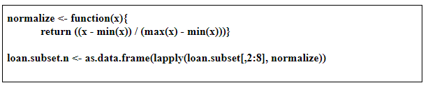
Step 3: Data Normalization
It’s very essential to always normalize the data set so that the output remains unbiased. In the below code snippet, we’re storing the normalized data set in the ‘loan.subset.n’ variable and also we’re removing the ‘Credibility’ variable since it’s the response variable that needs to be predicted.
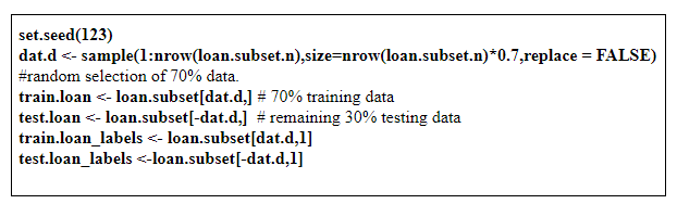
Step 4: Data Splicing
It basically involves splitting the data set into training and testing data sets. Then, it is necessary to create a separate data frame for the ‘Credibility’ variable so that our final outcome can be compared with the actual value.
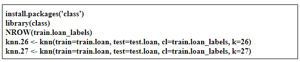
Step 5: Building a Machine Learning model
At this stage, we have to build a model by using the training data set. Since we’re using the KNN algorithm to build the model, we must first install the ‘class’ package provided by R. Next, we’re going to calculate the number of observations in the training data set.
Step 6: Model Evaluation
After building the model, it is time to calculate the accuracy of the created models:
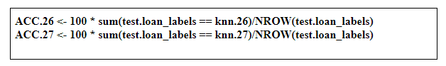
As shown above, the accuracy for K = 26 is 67.66 and for K = 27 it is 67.33. So, from the output, we can see that our model predicts the outcome with an accuracy of 67.67% which is good since we worked with a small data set.
The summarizing words…
KNN proves to be a useful algorithm at a lot many areas such as in banking sectors to predict whether a loan will be approved by a manager for an individual or not, in credit rate calculation of an individual by comparing the rate with a person bearing similar traits, and also in politics to classify a potential voter. Other areas in which KNN algorithms can be used are Speech Recognition, Handwriting Detection, Image Recognition and Video Recognition.


.svg)


