


1. What is Logistic Regression?
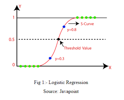
Logistic Regression is one of the machine learning algorithms used for solving classification problems. It is used to estimate probability whether an instance belongs to a class or not. If the estimated probability is greater than threshold, then the model predicts that the instance belongs to that class, or else it predicts that it does not belong to the class as shown in fig 1. This makes it a binary classifier. Logistic regression is used where the value of the dependent variable is 0/1, true/false or yes/no.
Example 1
Suppose we are interested to know whether a candidate will pass the entrance exam. The result of the candidate depends upon his attendance in the class, teacher-student ratio, knowledge of the teacher and interest of the student in the subject are all independent variables and result is dependent variable. The value of the result will be yes or no. So, it is a binary classification problem.

Example 2
Suppose we want to predict whether a person is suffering from Covid-19 or not. The symptoms of the patient include shortness of breath, muscle aches, sore throat, runny nose, headache and chest pain are all independent variables and presence of covid-19 (y) is dependent variable. The value of the dependent variable will be yes or no, true or false and 0 or 1.

2. Why Logistic Regression, Not Linear Regression
Linear Regression models the relationship between dependent variable and independent variables by fitting a straight line as shown in Fig 4.
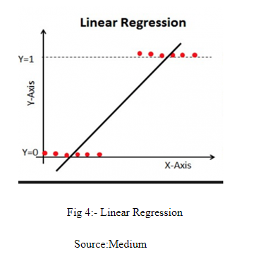
In Linear Regression, the value of predicted Y exceeds from 0 and 1 range. As discussed earlier, Logistic Regression gives us the probability and the value of probability always lies between 0 and 1. Therefore, Logistic Regression uses sigmoid function or logistic function to convert the output between [0,1]. The logistic function is defined as:
1 / (1 + e^-value)
Where e is the base of the natural logarithms and value is the actual numerical value that you want to transform. The output of this function is always 0 to 1.
The equation of linear regression is
Y=B0+B1X1+...+BpXp
Logistic function is applied to convert the output to 0 to 1 range
P(Y=1)=1/(1+exp(?(B0+B1X1+…+BpXp)))
We need to reformulate the equation so that the linear term is on the right side of the formula.
log(P(Y=1)/1?P(Y=1))= B0+B1X1+…+BpXp
where log(P(Y=1)/1?P(Y=1)) is called odds ratio.
3. Practical Implementation of Logistic Regression
Problem Statement: - In this problem, we want to predict if a person is suffering from heart disease or not.
Data Description:- To solve this problem, I have downloaded a heart disease dataset from Kaggle (https://www.kaggle.com/ronitf/heart-disease-uci) to predict if a person is having heart disease or not.
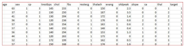
This dataset includes the various attributes like age, sex, chest pain type (cp), resting blood pressure (trestbps), serum cholestoral (chol), fasting blood sugar (fbs), resting electrocardiographic results (restecg), maximum heart rate achieved (thalach), exercise induced angina (exang), oldpeak, the slope of the peak exercise ST segment (slope), number of major vessels (0-3) colored by flourosopy (ca), thal and target. The value of the target is either 0 or 1 i.e. the person is having heart disease or not.
Implementation:-
First, we load a dataset heart.csv into R studio.
data<-read.csv("heart.csv")
Second, we partition the dataset into training and testing.
ind<-createDataPartition(data$target,p=.70,list = F)
training<-data[ind,]
testing<-data[-ind,]
Third, we create a model on the training dataset
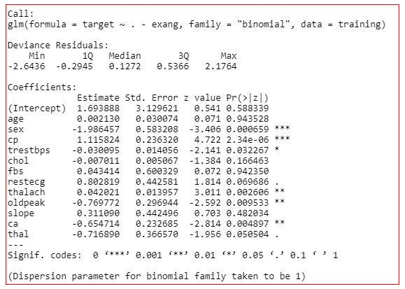
model<-glm(target~.,family="binomial",data=training)
summary(model)
Summary of the model
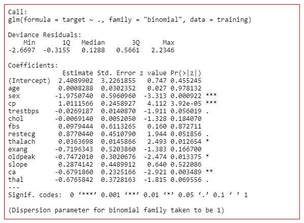
The summary of the model shows how significant the independent variables are. It shows that sex, cp, trestbps, restecg, thalach, oldpeak, ca and thal are significant variables and rest of the variables are not significant. But we will not remove the insignificant variables straight away. We will check the three more values in the summary-
AIC value,
Null deviance
and residual deviance.
Null deviance- It shows how well the response variable is predicted by a model that includes only intercept.
Residual deviance- It shows how well the response variable is predicted by a model that include all independent variables.
AIC- AIC provides a method for assessing the quality of your model through comparison of related models.
Optimizing the model
First, we will remove the age feature
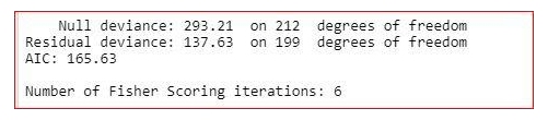
model<-glm(target~.-age,training,family="binomial")
summary(model)
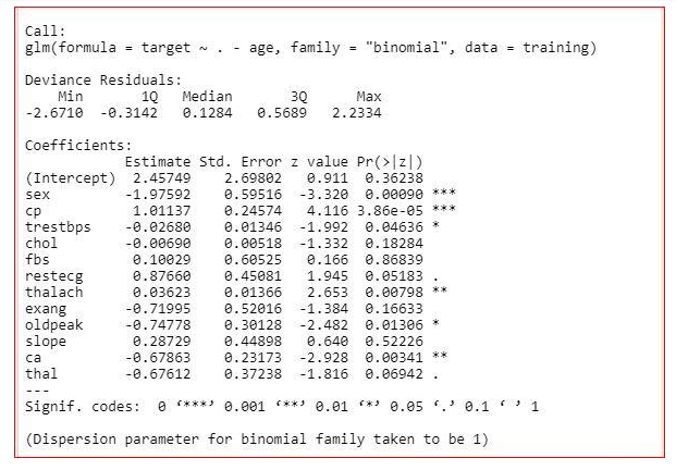
Here, we can see that AIC value got decreased. So, we can remove the age from the dataset.
Now, we will remove the chol variable from the dataset.
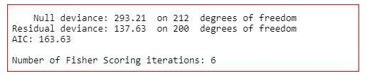
model<-glm(target~.-chol,training,family="binomial")
summary(model)
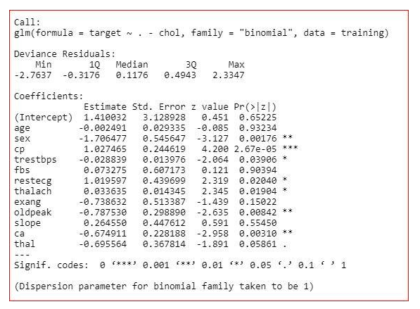
From the summary, we can see that the residual deviance is increasing, and AIC value is decreasing by a very small amount. So, we will not remove the chol variable.
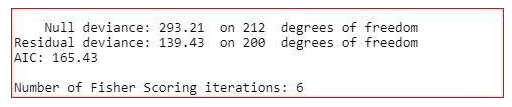
model<-glm(target~.-fbs,family="binomial",data=training)
summary(model)
From the summary, we can see that the value of AIC is decreasing. So, we will remove the fbs variable.
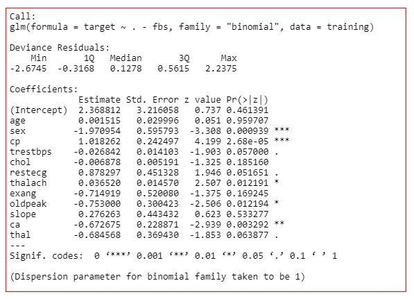
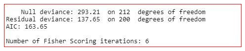
model<-glm(target~.-exang,family="binomial",data=training)
summary(model)
The summary shows that the value of Residual deviance is increasing, and AIC is also not decreasing much. So, we will not remove the exang variable.
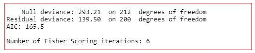
model<-glm(target~.-slope,family="binomial",data=training)
summary(model)
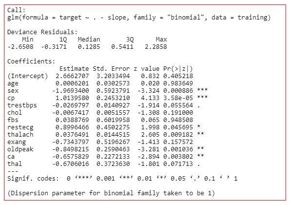
The summary shows that the value of residual deviance is increased and the value of AIC has not been decreased much. So, we will not remove the slope variable.
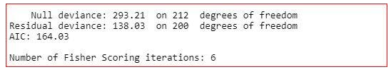
The final model is
model<-glm(target~.-age-fbs,family="binomial",data=training)
summary(model)
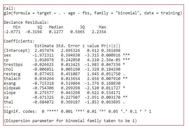

We have created the final model on the training data. Now, we will check the model on the testing data.
res<-predict(model,testing,type="response")
table(Actualvalue=testing$target,Predictedvalue=res>0.5)
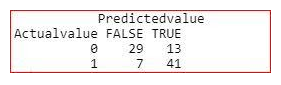
Accuracy of the model
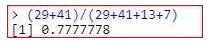
We need to reduce True Negatives in this case. Because, if a person is having heart disease and the model is predicting no, it may cost life.
4. How to find the threshold value
res<-predict(model,training,type="response")
library(ROCR)
ROCRPred=prediction(res,training$target)
ROCRPerf<-performance(ROCRPred,"tpr","fpr")
plot(ROCRPerf,colorize=TRUE,print.cutoffs.at=seq(0.1,by=0.1))
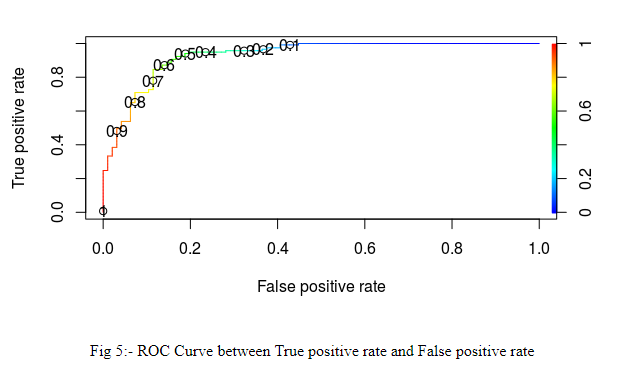
While selecting the threshold value, we should take care that true positive rate should be maximum and false negative rate should be minimum. Because, if a person is having disease, but the model is predicting that he is not having disease, it may cost someone’s life
The plot (Fig 5) shows that if we take threshold=0.4, true positive rate increase.
res<-predict(model,testing,type="response")
table(Actualvalue=testing$target,Predictedvalue=res>0.4)
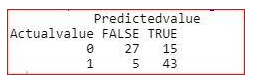
Here, we can see that the value of True negative decreases from 7 to 5.
Accuracy of the model
The accuracy of the model is coming the same if we use threshold value=0.4 or 0.5 but in case of threshold value=0.4, the true negative cases decrease. So, it is better to take 0.4 value as threshold value. The selection of threshold value depends upon the use case. In case of medical problems, our focus is to decrease true negatives because if a person is having disease, but the model is predicting that he is not having disease, it may cost someone’s life.


.svg)


